
Coastal Species Distribution Models
This tutorial will discuss how to run Species Distribution Models (SDMs) on coastal species using biomod2 in R. In this example we will use models to estimate the probability of occurence at two timepoints: present day and the Last Glacial Maximum (LGM). You can do the same with more time points, into the past and/or future.
We will obtain the predictor environmental variables from Bio-Oracle with the R package sdmpredictors. Since I work on intertidal species, I want to include both terrestrial and marine environmental variables. We will first load and stack the layers.
It is also important to only include variables that are available at both time points you want to model.
library(sdmpredictors)

# Download present day environmental variables
#+++++++++++++++++++++++++++++++++++++++++++++++++++++++++++++++++++++++


#download terrestrial features (Temp_max, Temp_min, Temp_range)
terr <- load_layers( layercodes = c("WC_bio5", "WC_bio6", "WC_bio7") , equalarea=FALSE, rasterstack=TRUE)

#download marine features
mar <- load_layers( layercodes = c("MS_biogeo08_sss_mean_5m", "MS_biogeo13_sst_mean_5m") , equalarea=FALSE, rasterstack=TRUE)

#check the chacteristics of each raster stack
terr
## class : RasterStack
## dimensions : 1800, 4320, 7776000, 3 (nrow, ncol, ncell, nlayers)
## resolution : 0.08333333, 0.08333333 (x, y)
## extent : -180, 180, -60, 90 (xmin, xmax, ymin, ymax)
## crs : +proj=longlat +datum=WGS84 +no_defs +ellps=WGS84 +towgs84=0,0,0
## names : WC_bio5, WC_bio6, WC_bio7
## min values : -7.3, -55.5, 5.3
## max values : 48.9, 25.8, 72.5mar## class : RasterStack
## dimensions : 2160, 4320, 9331200, 2 (nrow, ncol, ncell, nlayers)
## resolution : 0.08333333, 0.08333333 (x, y)
## extent : -180, 180, -90, 90 (xmin, xmax, ymin, ymax)
## crs : +proj=longlat +datum=WGS84 +no_defs +ellps=WGS84 +towgs84=0,0,0
## names : MS_biogeo08_sss_mean_5m, MS_biogeo13_sst_mean_5m
## min values : -0.05, -2.00
## max values : 40.43, 30.40Notice how the two raster stacks have different dimensions. In order to stack our terrestrial and marine rasters, we will need to resample them to have the same dimensions.
#Resample the marine by the terrestrial layers and stack into one raster stack

t<-extent(-180, 180, -90, 90) #layer extent from terrestrial stack
m<-extent(-180, 180, -90, 90) #layer extent from marine stack
#no need to edit the following 6 lines
extent_list<-list(t, m)
extent_list<-lapply(extent_list, as.matrix)
matrix_extent<-matrix(unlist(extent_list), ncol=length(extent_list))
rownames(matrix_extent)<-c("xmin", "ymin", "xmax", "ymax")
best_extent<-extent(min(matrix_extent[1,]), max(matrix_extent[3,]), min(matrix_extent[2,]), max(matrix_extent[4,]))
ranges<-apply(as.matrix(best_extent), 1, diff)

reso<-res(terr) #choose layer you want to keep resolution
nrow_ncol<-ranges/reso
s2<-raster(best_extent, nrows=nrow_ncol[2], ncols=nrow_ncol[1], crs=terr@crs) #choose layer crs you want to keep

t.2 <-resample(terr, s2, method="ngb") #resample terr by s2
m.2 <-resample(mar, s2, method="ngb") #resample mar by s2
env=stack(t.2, m.2) #stack resampled layers

# Set study extent
SA.ext <- extent(10, 40, -37, -22)

# Crop raster layer by extent & plot
env.c <- crop(env, SA.ext)
plot(env.c)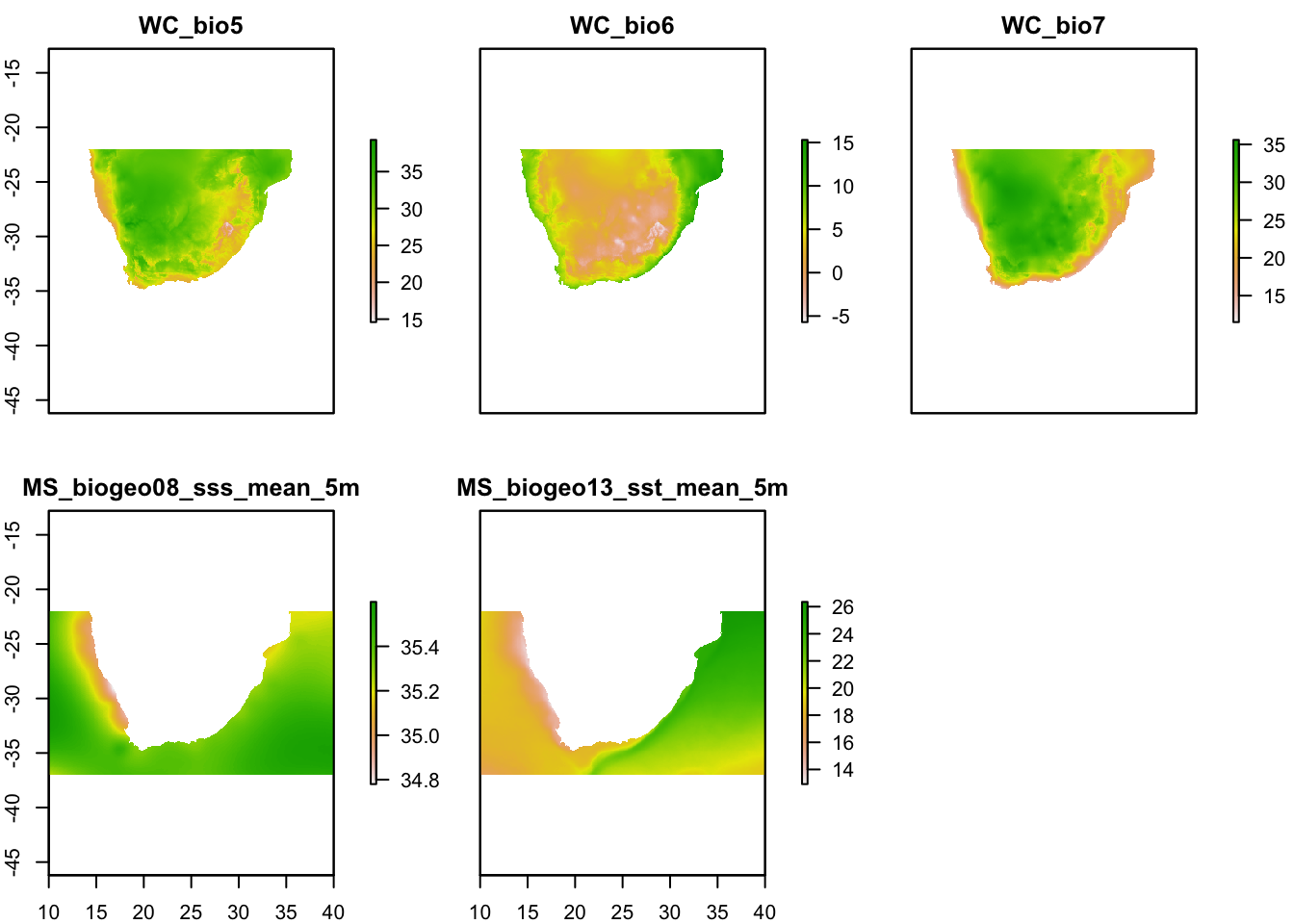
Plotting the environmental layers should give you a figure such as the above. Now we have a single raster stack called ‘env’. We now need to remove highly correlated environmental variables.
Here we will need to include our species presence data, which should include three columns: columns 1 & 2: x and y coordinates; column 3: presence (1) or absence (0) at each coordinate.
To check for variable collinearity, we will first extract the environmental data for each coordinate, create a correlation circle, and then calculate the variance inflation factor, or VIF.
# Filter environmental variables to account for collinearity
#+++++++++++++++++++++++++++++++++++++++++++++++++++++++++++++++++++++++

# Import your presence data and plot
pres.data <-read.table("Cpunctatus.pres2.txt",sep="\t",header=T)
plot(env.c$WC_bio5)
points(pres.data[,1:2], pch=19, col="black")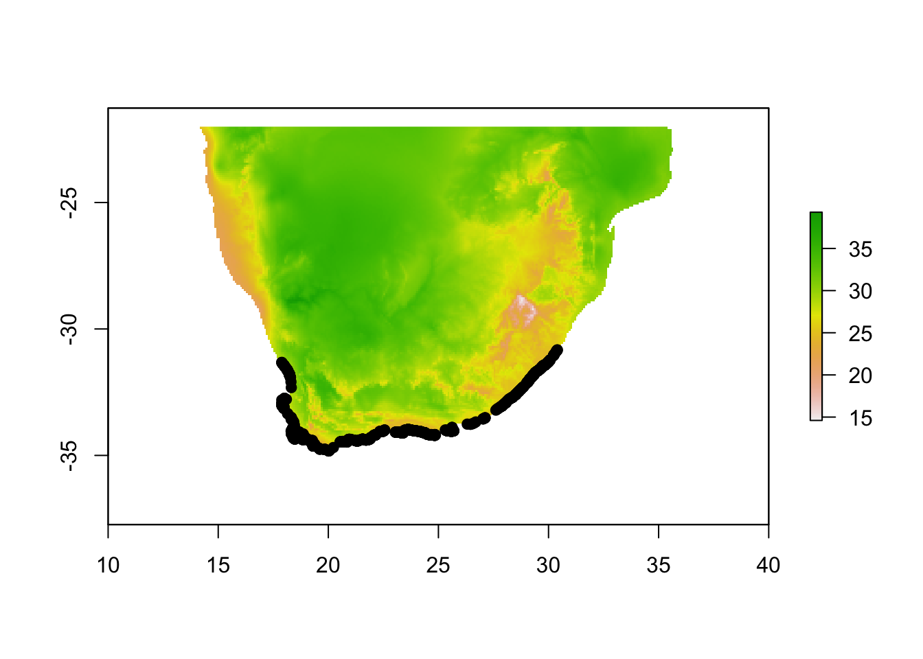
# Extract env values for our species locations:
envdata <- extract(x=env.c, y=cbind(pres.data$x, pres.data$y))

# Run PCA and plot correlation circle
# The `dudi.pca` function allows us to perform the PCA over the whole study area. We decide to keep only 2 principal component axes to summarize the whole environmental niche. NB: here be careful that none of your xy presence points are outside of the environmental raster layer, which will give NA values, which will give errors.

library(ade4)

pca1 <- dudi.pca(envdata, scannf = F, nf = 2)
round(pca1$eig/sum(pca1$eig)*100, 2)
## [1] 54.97 28.58 12.85 3.60# Plot the PCA to look for potential outliers in the environmental data.
plot(pca1$li[,1:2]) # PCA scores on first two axes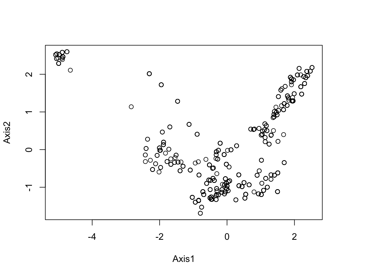
summary(pca1$li)## Axis1 Axis2
## Min. :-5.08541 Min. :-1.6900
## 1st Qu.:-0.69014 1st Qu.:-0.9985
## Median :-0.02031 Median :-0.3923
## Mean : 0.00000 Mean : 0.0000
## 3rd Qu.: 1.30403 3rd Qu.: 1.0404
## Max. : 2.52228 Max. : 2.5989# Plot a correlation circle.
s.corcircle(pca1$co)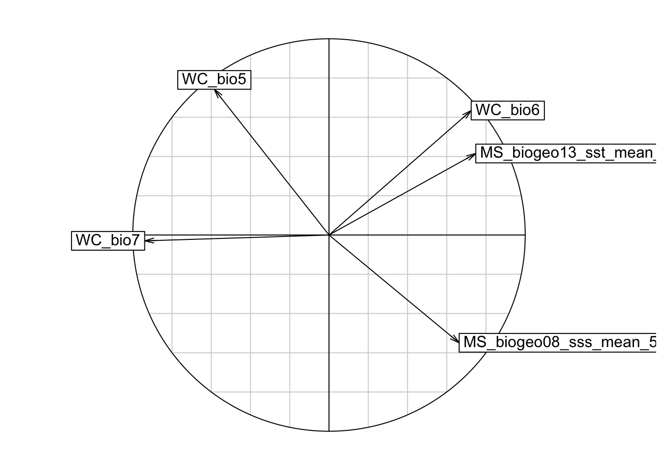
# From the correlation circle, we want to select variables on different axes and not in the same/overlapping environmental space. If there are multiple variables in the same quadrant of the circle, we should choose the one with a longer arrow, as that means it varies more over the environmental space, which is preferred. However, it is also important to know which environmental features are more relevant to your study species, and to choose according to the ecology of each species.

# A note on arrow directions: same direction = highly correlated, orthogonal (this means at a 90 degree angle) = unrelated, opposite directions = negatively correlated


# From the plot, we can get rid of variable WC_bio6, and plot again.

VARSEL <- c("WC_bio5", "WC_bio7", "MS_biogeo08_sss_mean_5m", "MS_biogeo13_sst_mean_5m") #select variables we want to keep
env.c.2 <- stack(subset(env.c, VARSEL)) #subset the rasterstack by the retained variables
envdata <- extract(x=env.c.2, y=cbind(pres.data$x, pres.data$y))
pca1 <- dudi.pca(envdata, scannf = F, nf = 2)
s.corcircle(pca1$co)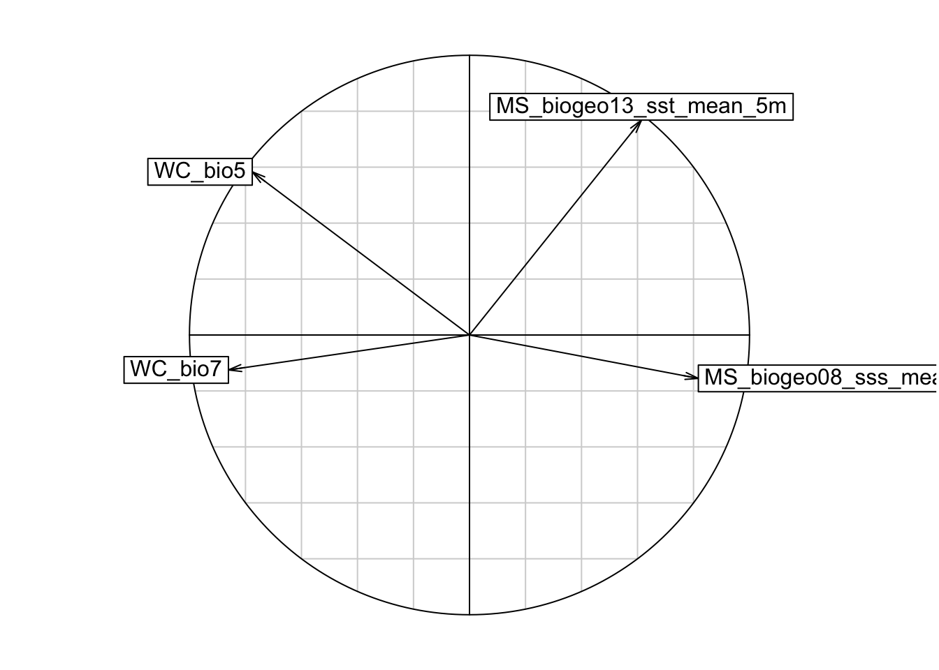
# Additionally assess the correlation with VIF
## Calculate variance inflation factor (VIF). Generally you want to exclude variables with a VIF>10.
library(usdm)

vif(env.c.2)
## Variables VIF
## 1 WC_bio5 13.712553
## 2 WC_bio7 5.311111
## 3 MS_biogeo08_sss_mean_5m 2.367307
## 4 MS_biogeo13_sst_mean_5m 9.803145#Since WC_bio5 has VIF > 10, then we will remove to create a final environmental raster stack for our models.
VARSEL2 <- c("WC_bio7", "MS_biogeo08_sss_mean_5m", "MS_biogeo13_sst_mean_5m") #select variables we want to keep
env.c.3 <- stack(subset(env.c.2, VARSEL2))
# We can write the raster stack to save in the home directory.
writeRaster(env.c.3, filename="env.current.tif", format="GTiff", overwrite=TRUE)Now that we have our final set of variables, we can download the same variables for the Last Glacial Maximum (LGM), 21,000 years ago. The environmental features from Bio-Oracle automatically include the lowered sea levels at the LGM which is nice.
It is generally good practice to include multiple climatic models. Here we will include two models: CCSM4 and MIROC. The oceanic layers are already an ensemble of multiple models, so we will use the ensemble without CCSM with the MIROC terrestrial layer, and the ocean model including CCSM with the CCSM terrestrial layer.
# Download historical environmental data
#+++++++++++++++++++++++++++++++++++++++++++++++++++++++++++++++++++++++


# Load layers and make sure they are in the same order as your contemporary raster stack (WC_bio5, WC_bio7, SSS, SST)

a.miroc.21 <- load_layers(layercodes = c("WC_bio7_cclgm"), equalarea=FALSE, rasterstack=TRUE,
                         datadir=NULL)

a.ccsm.21 <- load_layers(layercodes = c("WC_bio7_mrlgm"), equalarea=FALSE, rasterstack=TRUE,
                        datadir=NULL)

o.ens.adj.21 <- load_layers(layercodes = c("MS_biogeo08_sss_mean_21kya_adjCCSM", "MS_biogeo13_sst_mean_21kya_adjCCSM"), equalarea=FALSE, rasterstack=TRUE,
                       datadir=NULL)

o.ens.nc.21 <- load_layers(layercodes = c("MS_biogeo08_sss_mean_21kya_noCCSM", "MS_biogeo13_sst_mean_21kya_noCCSM"), equalarea=FALSE, rasterstack=TRUE,
                            datadir=NULL)

a.miroc.21.2 <-resample(a.miroc.21, s2, method="ngb")
a.ccsm.21.2 <-resample(a.ccsm.21, s2, method="ngb")
o.ens.adj.21.2 <-resample(o.ens.adj.21, s2, method="ngb")
o.ens.nc.21.2 <-resample(o.ens.nc.21, s2, method="ngb")

miroc.21 =stack(a.miroc.21.2, o.ens.nc.21.2 )
ccsm.21 =stack(a.ccsm.21.2, o.ens.adj.21.2 )

miroc.21.crop <- crop(miroc.21, SA.ext)
ccsm.21.crop <- crop(ccsm.21, SA.ext)

miroc.21.c <- stack(miroc.21.crop)
ccsm.21.c <- stack(ccsm.21.crop)

writeRaster(miroc.21.c, filename="miroc.21.tif", format="GTiff", overwrite=TRUE)
writeRaster(ccsm.21.c, filename="ccsm.21.tif", format="GTiff", overwrite=TRUE)
We are now ready to run our SDMs, using the package biomod2. We can use our environmental raster stack (for the present day) and presence data to create pseudo-absence data.
library(biomod2)

# Create presence and absence data
#+++++++++++++++++++++++++++++++++++++++++++++++++++++++++++++++++++++++

# Convert the column named "PRESENCE" to a character class
myResp<-as.numeric(pres.data$Cpunctatus)

myRespName <- 'Cpunctatus'

# Create presence and pseudo absences
SPC_PresAbs <- BIOMOD_FormatingData(resp.var = myResp,
                                    expl.var = env.c.3,
                                    resp.xy = pres.data[,c('x', 'y')],
                                    resp.name = myRespName,
                                    PA.nb.rep = 3,
                                    PA.nb.absences = 10000,
                                    PA.strategy = 'random')
##
## -=-=-=-=-=-=-=-=-=-=-=-=-= Cpunctatus Data Formating -=-=-=-=-=-=-=-=-=-=-=-=-=
##
## ! No data has been set aside for modeling evaluation
## > Pseudo Absences Selection checkings...
## > random pseudo absences selection
## > Pseudo absences are selected in explanatory variables
## ! Some NAs have been automaticly removed from your data
## -=-=-=-=-=-=-=-=-=-=-=-=-=-=-=-=-=-= Done -=-=-=-=-=-=-=-=-=-=-=-=-=-=-=-=-=-=## NOTE: if you get an error that looks like this:
## 'Error in .BIOMOD_FormatingData.check.args(resp.var, expl.var, resp.xy, : Explanatory variable must be one of numeric, data.frame, matrix, RasterLayer, RasterStack, SpatialPointsDataFrame, SpatialPoints'
#Then simply re-create your raster stack and try again. As such:
env.c.2 <- stack(env.c.2)
SPC_PresAbs <- BIOMOD_FormatingData(resp.var = myResp,
expl.var = env.c.3,
resp.xy = pres.data[,c('x', 'y')],
resp.name = myRespName,
PA.nb.rep = 3,
PA.nb.absences = 10000,
PA.strategy = 'random') ##
## -=-=-=-=-=-=-=-=-=-=-=-=-= Cpunctatus Data Formating -=-=-=-=-=-=-=-=-=-=-=-=-=
##
## ! No data has been set aside for modeling evaluation
## > Pseudo Absences Selection checkings...
## > random pseudo absences selection
## > Pseudo absences are selected in explanatory variables
## ! Some NAs have been automaticly removed from your data
## -=-=-=-=-=-=-=-=-=-=-=-=-=-=-=-=-=-= Done -=-=-=-=-=-=-=-=-=-=-=-=-=-=-=-=-=-=# Check the number of absences
SPC_PresAbs##
## -=-=-=-=-=-=-=-=-=-=-=-=-= 'BIOMOD.formated.data.PA' -=-=-=-=-=-=-=-=-=-=-=-=-=
##
## sp.name = Cpunctatus
##
## 1163 presences, 0 true absences and 323 undifined points in dataset
##
##
## 3 explanatory variables
##
## WC_bio7 MS_biogeo08_sss_mean_5m MS_biogeo13_sst_mean_5m
## Min. :11.50 Min. :34.78 Min. :12.97
## 1st Qu.:14.30 1st Qu.:35.30 1st Qu.:16.39
## Median :16.40 Median :35.33 Median :18.35
## Mean :16.26 Mean :35.27 Mean :18.52
## 3rd Qu.:17.50 3rd Qu.:35.34 3rd Qu.:21.04
## Max. :22.30 Max. :35.38 Max. :26.01
##
##
## 3 Pseudo Absences dataset available ( PA1 PA2 PA3 ) with 151
## absences in each (true abs + pseudo abs)
##
## -=-=-=-=-=-=-=-=-=-=-=-=-=-=-=-=-=-=-=-=-=-=-=-=-=-=-=-=-=-=-=-=-=-=-=-=-=-=-=-=## Notice how the output here says that there are a different number of pseudo absences than you input in the 'PA.nb.absences' parameter. I am guessing this is because the same cell can be chosen as an absence over and over within this step, so I would advise playing with that parameter until you get roughly and equal amount of absences as you have presences.
# Plot your pseudo absences
plot(SPC_PresAbs)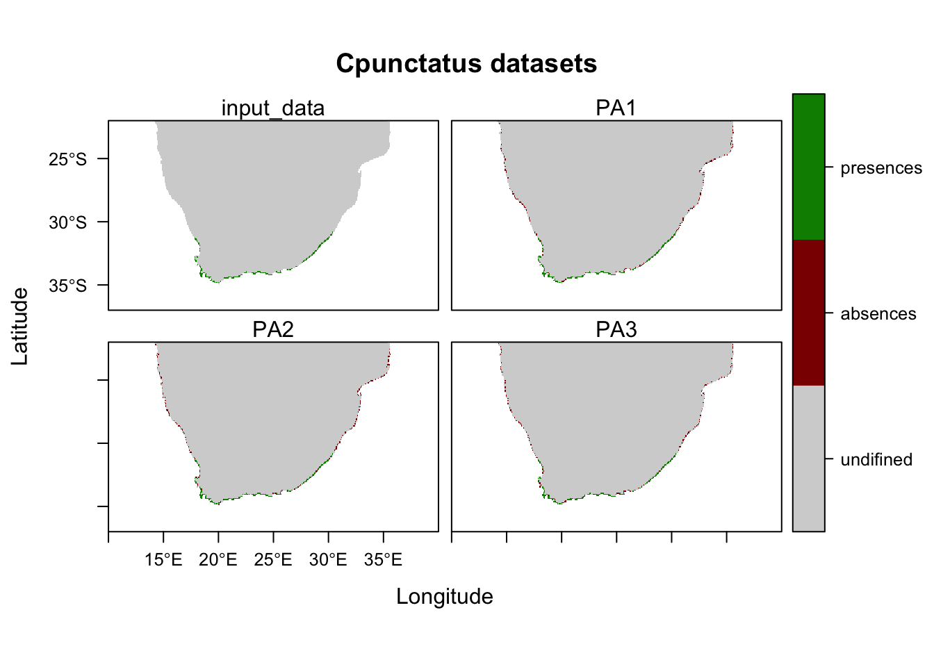
Next we will run model models using our presence and pseudo absence data and environmental features. Here we will run 6 different models, over 10 runs, using 30% of the data for callibration, and 70% for fitting models.
We will then check how well the model performs with two separate evalution scores: ROC and TSS. Generally, a ROC > 0.8 and TSS > 0.55 are indicative of high model accuracy.
# Run BIOMOD Models
#+++++++++++++++++++++++++++++++++++++++++++++++++++++++++++++++++++++++
# Set modeling options (NB: refer to the package vingette for non-default model options)
MySpc_options <- BIOMOD_ModelingOptions(
  GLM = list( type = 'quadratic', interaction.level = 1 ),
  GBM = list( n.trees = 1000 ),
  GAM = list( algo = 'GAM_mgcv' ) )

# Run the models with specific parameters.
MySpc_models <- BIOMOD_Modeling( data = SPC_PresAbs,
                                 models = c("GLM","GAM", "GBM", "RF","MARS", "FDA"),
                                 models.options = MySpc_options,
                                 NbRunEval = 10,
                                 DataSplit = 70,
                                 VarImport = 3,
                                 models.eval.meth=c('TSS','ROC'),
                                 do.full.models = F )

# Get models evaluation scores
#+++++++++++++++++++++++++++++++++++++++++++++++++++++++++++++++++++++++
MyModels_scores <- get_evaluations(MySpc_models)

MyModels_scores["ROC","Testing.data",,,]
MyModels_scores["TSS","Testing.data",,,]

# Graphically see model scores
models_scores_graph(MySpc_models, by = "models" , metrics = c("ROC","TSS"), xlim = c(0.5,1), ylim = c(0.5,1))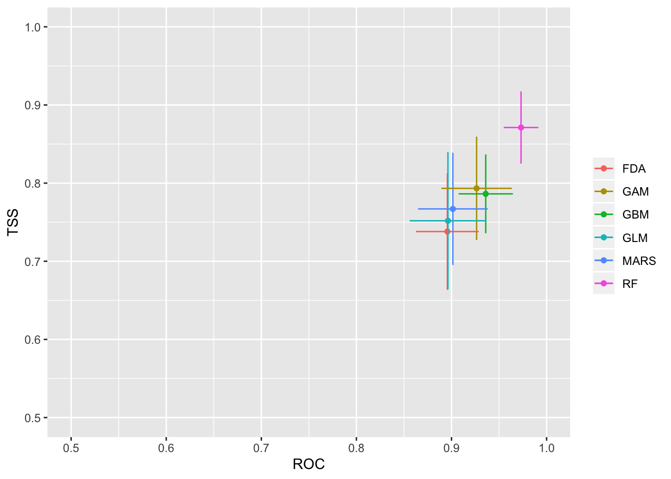
models_scores_graph(MySpc_models, by = "cv_run" , metrics = c("ROC","TSS"), xlim = c(0.5,1), ylim = c(0.5,1))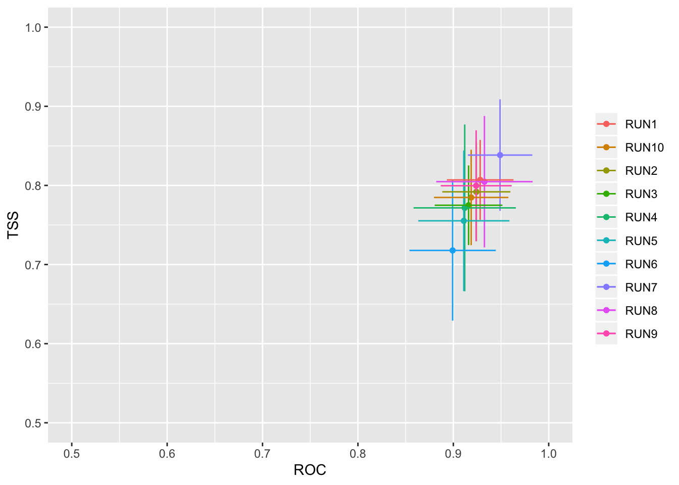
models_scores_graph(MySpc_models, by = "data_set" , metrics = c("ROC","TSS"), xlim = c(0.5,1), ylim = c(0.5,1))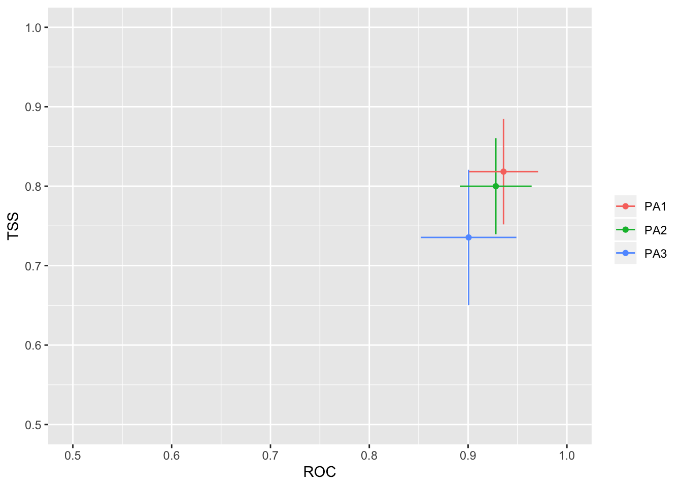
We can also look at the importance of each environmental variable in explaining the distribution, which is calculated as the variable importance.
# Variable importance in models
#+++++++++++++++++++++++++++++++++++++++++++++++++++++++++++++++++++++++

# Calculate variable importance. The higher a score is, the more important is the variable. We will visualize this as a barplot.

MyModels_var_import <- get_variables_importance(MySpc_models)
dimnames(MyModels_var_import)
## [[1]]
## [1] "WC_bio7" "MS_biogeo08_sss_mean_5m"
## [3] "MS_biogeo13_sst_mean_5m"
##
## [[2]]
## [1] "GLM" "GAM" "GBM" "RF" "MARS" "FDA"
##
## [[3]]
## [1] "RUN1" "RUN2" "RUN3" "RUN4" "RUN5" "RUN6" "RUN7" "RUN8" "RUN9"
## [10] "RUN10"
##
## [[4]]
## Cpunctatus_PA1 Cpunctatus_PA2 Cpunctatus_PA3
## "PA1" "PA2" "PA3"# Average variable importance by algorithm
mVarImp <- apply(MyModels_var_import, c(1,2), median)
mVarImp <- apply(mVarImp, 2, function(x) x*(1/sum(x))) # standardize the data
mVarImp ## GLM GAM GBM RF MARS
## WC_bio7 0.2578125 0.1979434 0.1516144 0.1860687 0.2718195
## MS_biogeo08_sss_mean_5m 0.3320313 0.4531766 0.7033224 0.4394084 0.4386095
## MS_biogeo13_sst_mean_5m 0.4101563 0.3488799 0.1450632 0.3745229 0.2895710
## FDA
## WC_bio7 0.1478463
## MS_biogeo08_sss_mean_5m 0.4384944
## MS_biogeo13_sst_mean_5m 0.4136593#save as table
write.table(mVarImp, file="modelVarImp.txt", sep="\t", quote = FALSE)It is also good practice to visualize the response curves pertaining to each environmental variable.
# Response curves
#+++++++++++++++++++++++++++++++++++++++++++++++++++++++++++++++++++++++

# To analyze how each environmental variable influences modelled probability of species presence, we will use an evaluation procedure proposed by Elith et al.(2005).

# A plot of these predictions allows visualisation of the modeled response(y-axis) to the given variable (x-axis),conditional to the other variables being held constant.

# Here I will show the response curves for the RF model, but you can do this for all models:

MySpc_rf  <- BIOMOD_LoadModels(MySpc_models, models='RF')

rf_eval_strip <- biomod2::response.plot2(
  models  = MySpc_rf, Data = get_formal_data(MySpc_models,'expl.var'),
  show.variables= get_formal_data(MySpc_models,'expl.var.names'),
  do.bivariate = FALSE, fixed.var.metric = 'median', legend = FALSE,
  display_title = FALSE, data_species = get_formal_data(MySpc_models,'resp.var'))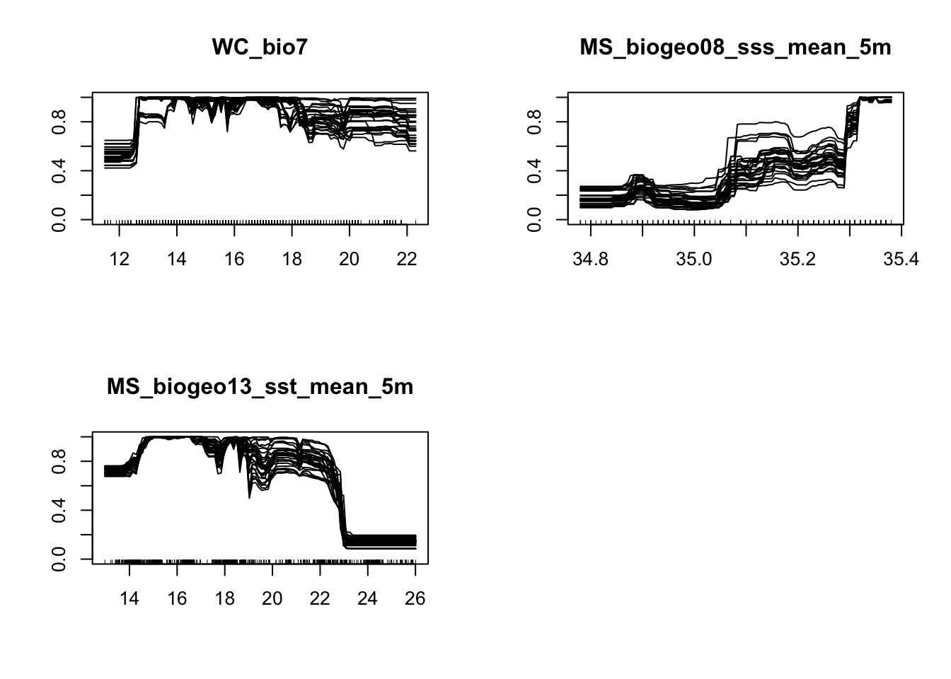
Now we will project our models onto the current climate, and see how well they predict the current distribution. Running this script will create a folder in your directory called ‘current’. Note that this will automatically overwrite any other folder of the same name.
Afterwards we will create the ensemble model, which will combine the 6 model types we specified earlier. Here we will use a TSS cut off of 0.55 and ROC cut off of 0.8.
# Map individual models onto the current Southern African climate
#+++++++++++++++++++++++++++++++++++++++++++++++++++++++++++++++++++++++

MySpc_models_proj_current <- BIOMOD_Projection( modeling.output = MySpc_models,
                                                new.env = env.c.3,
                                                proj.name = "current",
                                                binary.meth = "ROC",
                                                output.format = ".img",
                                                do.stack = FALSE )


# Plot and compare the maps for the potential current distribution projected by the different models.
plot(MySpc_models_proj_current,  str.grep="PA1_RUN1")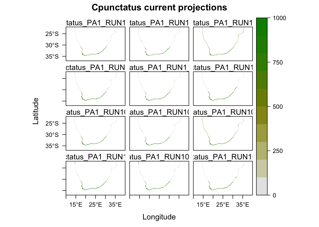
# If any of the models over or under estimate the distribution, then you can consider leaving them out of the ensemble model.


# Run ensemble models
#+++++++++++++++++++++++++++++++++++++++++++++++++++++++++++++++++++++++

MySpc_ensemble_models <- BIOMOD_EnsembleModeling( modeling.output = MySpc_models,
                                                  chosen.models ='all',
                                                  em.by = 'all',  #combine all models
                                                  eval.metric = 'all',
                                                  eval.metric.quality.threshold = c(0.55,0.8),
                                                  models.eval.meth = c('TSS','ROC'),
                                                  prob.mean = FALSE,
                                                  prob.cv = TRUE, #coefficient of variation across predictions
                                                  committee.averaging = TRUE,
                                                  prob.mean.weight = TRUE,
                                                  VarImport = 0 )

# Check ensemble scores
MySpc_ensemble_models_scores <- get_evaluations(MySpc_ensemble_models)
MySpc_ensemble_models_scores


# Ensemble model forecast onto current environment
#+++++++++++++++++++++++++++++++++++++++++++++++++++++++++++++++++++++++
MySpc_ensemble_models_proj_current <- BIOMOD_EnsembleForecasting(
  EM.output = MySpc_ensemble_models,
  projection.output = MySpc_models_proj_current,
  binary.meth = "ROC",  #make binary predictions (pres/abs) based on ROC score
  output.format = ".img",
  do.stack = FALSE )

# The projections for current conditions are stored in the 'proj_current' directory.
get_projected_models(MySpc_ensemble_models_proj_current)

# Plot them all
plot(MySpc_ensemble_models_proj_current)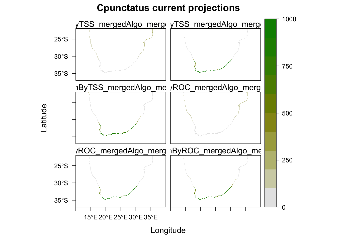
plot(MySpc_ensemble_models_proj_current, str.grep="EMcaByTSS")
plot(MySpc_ensemble_models_proj_current, str.grep="EMwmeanByTSS")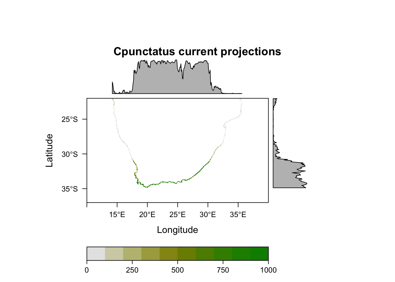
# Ensemble model hindcast onto LGM environment
#+++++++++++++++++++++++++++++++++++++++++++++++++++++++++++++++++++++++
#Fit model using new environmental variables

#First we need to re-name the raster stack layers to be the same as the 'present-day' raster stack we built the model on
names(miroc.21.c) <- c('WC_bio7','MS_biogeo08_sss_mean_5m', 'MS_biogeo13_sst_mean_5m')

#Then project the model onto the new environmental layers
MySpc_models_proj_LGM1 <- BIOMOD_Projection( modeling.output = MySpc_models,
                                             new.env = miroc.21.c,
                                             proj.name = "miroc.LGM",
                                             binary.meth = c("ROC"),
                                             output.format = ".img",
                                             do.stack = FALSE)


#Then run hindcasting ensemble model:
 MySpc_ensemble_models_proj_LGM1 <- BIOMOD_EnsembleForecasting(
   EM.output = MySpc_ensemble_models,
   projection.output = MySpc_models_proj_LGM1,
   binary.meth = "ROC",
   output.format = ".img",
   do.stack = FALSE,
   build.clamping.mask=F)

# Then do this same for CCSM LGM layers
names(ccsm.21.c) <- c('WC_bio7','MS_biogeo08_sss_mean_5m', 'MS_biogeo13_sst_mean_5m')
MySpc_models_proj_LGM2 <- BIOMOD_Projection( modeling.output = MySpc_models,
                                             new.env = ccsm.21.c,
                                             proj.name = "ccsm.LGM",
                                             binary.meth = c("ROC"),
                                             output.format = ".img",
                                             do.stack = FALSE)

 MySpc_ensemble_models_proj_LGM2 <- BIOMOD_EnsembleForecasting(
   EM.output = MySpc_ensemble_models,
   projection.output = MySpc_models_proj_LGM2,
   binary.meth = "ROC",
   output.format = ".img",
   do.stack = FALSE,
   build.clamping.mask=F)
Finally, we can map the outputs of the models to create a single figure in which they are compared. We will first combine the MIROC and CCSM model outputs, by averaging their values per cell. We will also enlargen the cells to make the output maps easier to read.
## Plotting SDM outputs
#+++++++++++++++++++++++++++++++++++++++++++++++++++++++++++++++++++++++

library(rasterVis)
library(gridExtra)
library(rgdal)

cc = colorRampPalette( c("red", "white","blue"))

## Retreive output maps from the different directories
MyBinCP_curr <- raster::stack("Cpunctatus/proj_current/individual_projections/Cpunctatus_EMcaByTSS_mergedAlgo_mergedRun_mergedData.img")
MyBinCP_c.LGM <- raster::stack("Cpunctatus/proj_ccsm.LGM/individual_projections/Cpunctatus_EMcaByTSS_mergedAlgo_mergedRun_mergedData.img")
MyBinCP_m.LGM <- raster::stack("Cpunctatus/proj_miroc.LGM/individual_projections/Cpunctatus_EMcaByTSS_mergedAlgo_mergedRun_mergedData.img")

# Load a shapefile to have as a background map. You can find shapefiles either on the web or from R packages such as 'rnaturalearth'
SAmap <- readOGR("Cpunctatus/Africa.shp")
## OGR data source with driver: ESRI Shapefile
## Source: "/Users/ericaspotswoodnielsen/Desktop/website/SDM.tutorial/Cpunctatus/Africa.shp", layer: "Africa"
## with 762 features
## It has 3 fieldsSAmap.c <- crop(SAmap, SA.ext)
# Make ensemble output maps by combining the miroc and ccsm models (by averaging cell values)
CP.mean.LGM <- merge(MyBinCP_c.LGM, MyBinCP_m.LGM)
# Aggregate the cells to make the output more visable (this doubles the size of the cells)
CP.mean.LGM.agg <- aggregate(CP.mean.LGM, fact=2)
MyBinCP_c.agg <- aggregate(MyBinCP_curr, fact=2)
# Stack the current and LGM output layers
CP.sdms <- stack(MyBinCP_c.agg, CP.mean.LGM.agg)
names(CP.sdms) <- c('Current', 'LGM')
#Plot the current and LGM rasters in single plot
levelplot(CP.sdms, col.regions=cc, layout=c(1, 2)) + layer(sp.polygons(SAmap.c, fill='white', alpha=0.2))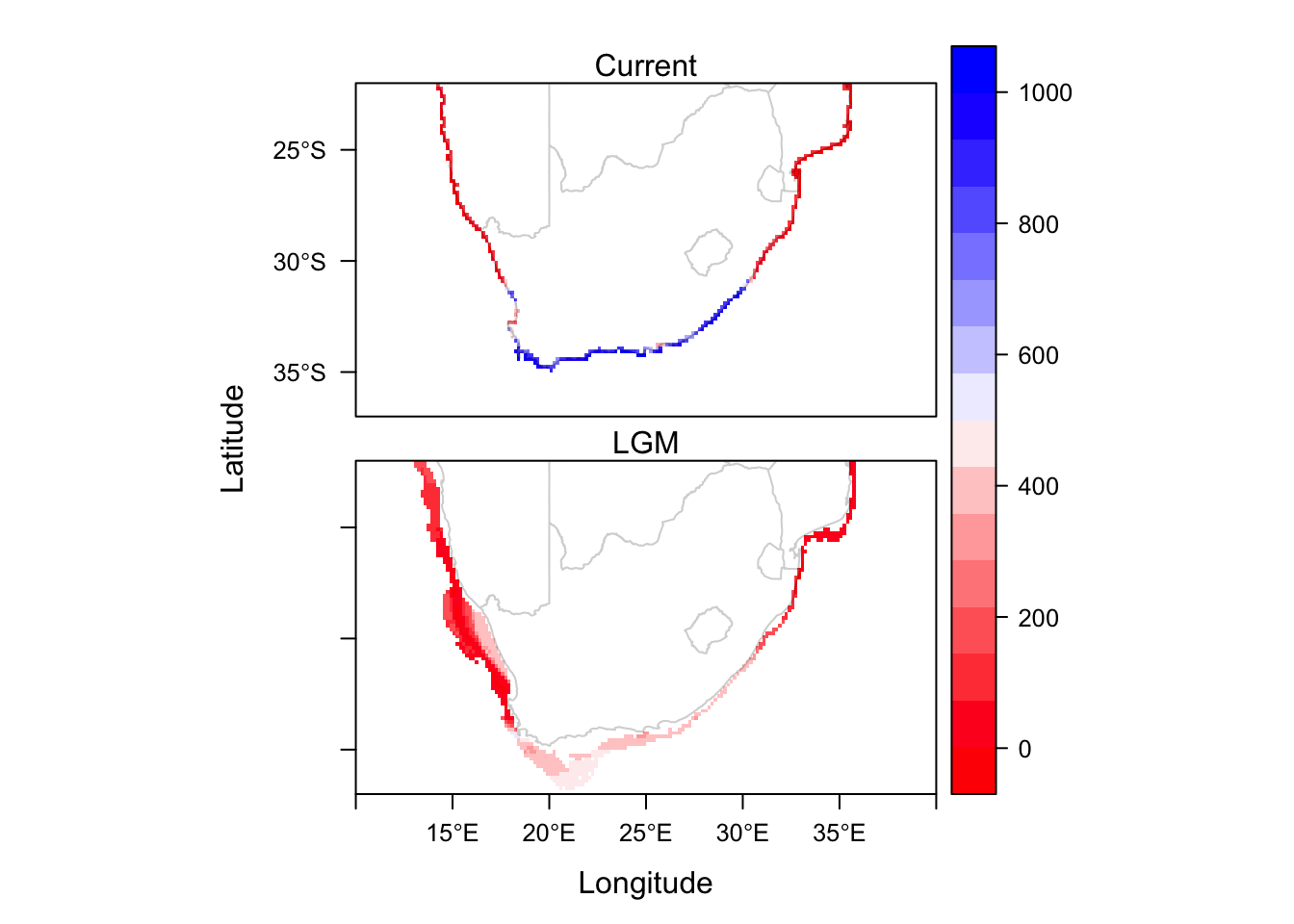
And here we have the final product, showing the average habitat suitability at two timepoints.
Thanks for reading, and feel free to let me know if you have any questions!
Post written by Erica Nielsen, R scripts written by Nikki Phair and Erica Nielsen.