
Population structure & outlier detection for Pool-seq data
This tutorial will discuss how to call SNPs and assess population structure from Pool-Seq data. Specifically, it will go through how to take a sync file from Popoolation, call SNPs with PoolFstat, filter SNPs to account for linkage disequilibrium, and infer population differentiation and identify outliers with BayPass.
To start, we need a sync file, which I generated using Popoolation2.
We will use this as the input for PoolFstat.
Note in all of the scripts below I will have the heading ‘SG’ just to indicate the species name.
################################# USING POOLFSTAT ###############################
##################################################################################

library(poolfstat)
library("WriteXLS")

##### Convert sync file to poolfstat file, and call SNPS

# We first have to give haploid sizes of each pool. Here, I had mostly 40 individuals per pool, and since I am working with diploid species, we multiply that by 2,  to get 80 individuals for most pools.
psizes <- as.numeric(c('80', '80', '80', '80', '80', '80', '80', '80', '78', '80', '80', '80', '80', '60'))

# Then we give the names of each pool/sample.
pnames <- as.character(c('PN', 'HB', 'BB', 'LB', 'JB', 'SP', 'BT', 'CA', 'MB', 'KY', 'CF', 'PA', 'HH', 'HL'))

# Here is where we read the sync file and call SNPs. The input file must have the '.sync' extension, and can also be gzipped, like in the example below. The parameters to note are:

#1) min.rc =  the minimum # reads that an allele needs to have (across all pools) to be called
#2) min.cov.per.pool = the minimum allowed read count per pool for SNP to be called
#3) max.cov.per.pool = the maximum read count per pool for SNP to be called
#4) min.maf = the minimum allele frequency (over all pools) for a SNP to be called (note this is obtained from dividing the read counts for the minor allele over the total read coverage)
#5) nlines.per.readblock = number of lines in sync file to be read simultaneously

SG.pooldata <- popsync2pooldata(sync.file = "SG.dn.b.sync.gz", poolsizes = psizes, poolnames = pnames,
                                     min.rc = 4, min.cov.per.pool = 20, max.cov.per.pool = 400,
                                     min.maf = 0.01, noindel = TRUE, nlines.per.readblock = 1e+06)

##### From this file we can compute global and per SNP FSTs
SG.snp.fsts <- computeFST(SG.pooldata, method = "Anova", snp.index = NA)

##### And we can compute pairwise FSTs
SG.pair.fst <- computePairwiseFSTmatrix(SG.pooldata, method = "Anova",
                                        min.cov.per.pool = 20, max.cov.per.pool = 400,
                                        min.maf = 0.01,
                                        output.snp.values = FALSE)

##### If you want to save the pairwise matrix, you can do the following:
SG.p.fst <- SG.pair.fst$PairwiseFSTmatrix
SG.p.fst <- as.data.frame(SG.p.fst)
WriteXLS(SG.p.fst, "SG.p.fst.xls")

###### Next, we will convert the poolfstat file to BayPass input files

#### Here you get three output files = genobaypass (allele counts), poolsize (haploid size per pool), & snpdet (snp info matrix). These will automatically be written in your working directory. Note the subsample size here can be used to sample to a smaller number of SNPs. If the subsample size is <0, then all SNPs are included in the BayPass files.
pooldata2genobaypass(SG.pooldata, writing.dir = getwd(), subsamplesize = -1)
From here, you may want to filter the SNP dataset to account for linkage disequilibrium. If so, you can use this custom script that randomly selects one SNP per every 1000 base pairs along each contig:
################################# LD PRUNING ###############################
##################################################################################

# To run the script below, you need to take the snpdet output from the poolfstat2baypass command above, and give the columns headers. Importantly, the first column must be titled "scaffold" and the second column must be titled "pos" (these are the contig and position columns).Here I called this file 'snpdet.pruning.txt'

# Read input file
data<-read.table("snpdet.pruning.txt",sep="\t",header=T)

# Initiate data for LD pruning
data_LD<-NULL

# Window for LD pruning, here at 1000 bp (select 1 SNP per 1000 base pairs)
window<-1000

# Print every unique contig, and for every contig, randomly subsample 1 SNP per 1000 bp window
scaffold_ID<-unique(data$scaffold)
for(i in 1:length(scaffold_ID)){
  print(scaffold_ID[i])
  subset<-data[which(data$scaffold==scaffold_ID[i]),]
for(j in 0:10){
  print(window*j+1)
  subset_bin_i<-subset[which(subset$pos>=window*j & subset$pos<=window*(j+1)),]
  random<-sample(1:length(subset_bin_i[,1]),1)
  subsubset<-subset_bin_i[random,]
  data_LD<-rbind(data_LD,subsubset)
}
}

# Get the unique LD pruned SNP list
uniq.LD <- unique(data_LD)

# Write to excel file
WriteXLS(uniq.LD, "SG.LD.list.xls")

####### SUBSET BAYPASS FILE  ###########

# Here we are going to filter our BayPass input files to now only relate to the LD-pruned SNPs. To do this, we first need to combine the .genobaypass and .snpdet outptut files from above. So in excel or text editor, have the first columns relate to the .snpdet output, then add the .genobaypass columns following. In other words, your input file here is the contig position, allele states, and then allele counts. Make sure the columns do not have headers. Here I called this file 'SG.snpdet.geno.txt'

library(dplyr)

# Read the .genobaypass/.snpdet file type explained above, relating to all SNPs
snp.data<-read.table("SG.snpdet.geno.txt",sep="",header=F)

# Read your LD SNP list. To make this text file, I just took the first two columns of the SG.LD.list excel file just created, and turned that into a text file. So basically a text file with first column being contig, and second column being position for all LD-pruned SNPs (but with no column headers)
ld.data<-read.table("SG.LD.index.txt",sep="\t",header=F)

# Filter the list of all SNPs to now only list the LD pruned SNPs
snp.data.f <- dplyr::inner_join(snp.data, ld.data)

# Write out as new file, and then from there you can split back up into new .snpdet and .genobaypass input files
write.table(snp.data.f, file="SG.LD.snpdet.geno.txt", col.names = F, row.names= F, quote = F)
Now we are ready to input our LD-pruned BayPass files into BayPass. Here we will use a combination of bash and R scripts to run through BayPass analyses. I will briefly show the main commands used in the bash scripts, and explain how they are used in combination with the R scripts.
The first step is to make sure you have compiled BayPass and have it with all of your input files in your working directory (not in R directory but Terminal type of program). Then you need to understand which of the model types you want to run. The standard core model is used to asses population structure, and identify outlier SNPs using a ‘FST type approach’. Alternatively, the auxiliary covariate model can be used to identify outlier SNPs using a ‘GEA type approach’, similar to BayEnv. Here we will just use the core model. The bash script will look something like this:
g_baypass -npop 14 -gfile SG.genobaypass -poolsizefile SG.poolsize -d0yij 8 -outprefix SG.BP -npilot 100
Here’s some parameter explanations:
-npop = number of pools
-gfile & -poolsizefiles are relating to your input file names
-d0yij = is something to do with the initial read counts and their distribution seeded into the model, and is specifically for Pool-seq data. I followed the tip in the manual that says to set it to 1/5th of the minimum pool size
-outprefix = the header of the output files
-npilot = number of pilot runs
So after you run the above, you should then get a number of output files. What we will need for the next part in R, is the following: ’_mat_omega.out’, ’_summary_beta_params.out’, ’_summary_pi_xtx.out’. You also need to make sure you have the ‘baypass_utils.R’ R code that comes with the program, as we will be running some of these scripts now.
Now we will go into R, to both visualize the results, but also to create the pseudo observation dataset (POD), which will be used to identify outlier SNPs.
################################# BAYPASS CREATE POD ###############################
##################################################################################

source("baypass_utils.R")
require(corrplot) ; require(ape)
library(WriteXLS)

# Read omega matrix BayPass output
SG.omega=as.matrix(read.table("SG.BP_mat_omega.out"))

# Identify pool names for plotting
colnames(SG.omega) <- c("PN","HB","BB","LB","JB","SP","BT","CA","MB",
            "KY","CF","PA","HH", "HL")
rownames(SG.omega) <- c("PN","HB","BB","LB","JB","SP","BT","CA","MB",
            "KY","CF","PA","HH", "HL")

# Create a correlation matrix of the omega values, which can be used to assess genomic differentiation between pools
cor.mat=cov2cor(SG.omega)
corrplot(cor.mat,method="color",mar=c(2,1,2,2)+0.1,
         main=expression("Correlation map based on"~hat(Omega)))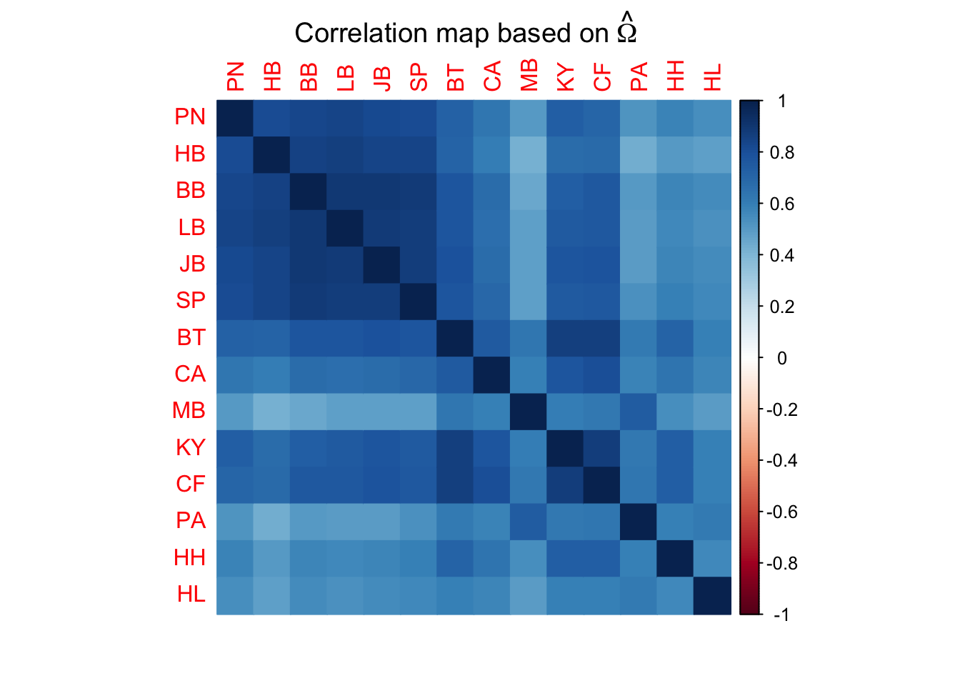
# We can also assess population differentiation with hierarchical clustering:
bta14.tree=as.phylo(hclust(as.dist(1-cor.mat**2)))
plot(bta14.tree,type="p",
     main=expression("Hier. clust. tree based on"~hat(Omega)~"("*d[ij]*"=1-"*rho[ij]*")"))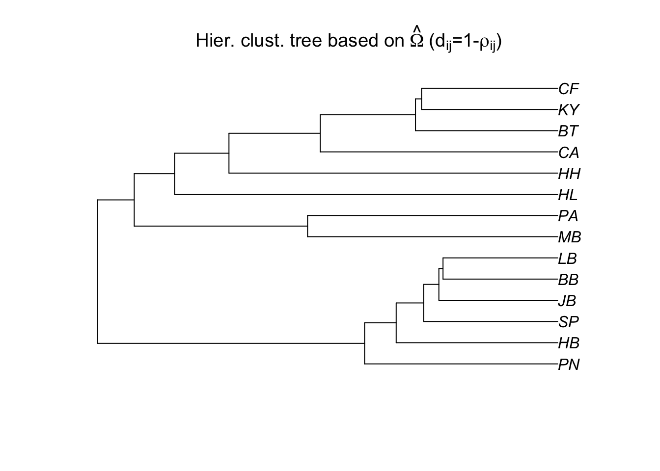
# Read the xtx BayPass output
SG.snp.res=read.table("SG.BP_summary_pi_xtx.out",h=T)

# Get the Pi Beta distribution for POD generation
SG.pi.beta.coef=read.table("SG.BP_summary_beta_params.out",h=T)$Mean

# Upload original data to get read counts
SG.data<-geno2YN("SG.genobaypass")

# Simulate POD dataset to use for outlier SNP detection
simu.SG <-simulate.baypass(omega.mat=SG.omega,nsnp=10000,sample.size=SG.data$NN,
                           beta.pi=SG.pi.beta.coef,pi.maf=0,suffix="SG.BP.sim")
## 1000 SNP simulated out of 10000
## 2000 SNP simulated out of 10000
## 3000 SNP simulated out of 10000
## 4000 SNP simulated out of 10000
## 5000 SNP simulated out of 10000
## 6000 SNP simulated out of 10000
## 7000 SNP simulated out of 10000
## 8000 SNP simulated out of 10000
## 9000 SNP simulated out of 10000
## 10000 SNP simulated out of 10000The above R script will give you new BayPass input files with the suffix of ‘SG.BP.sim’. We will now run BayPass again with these new gfile, using a bash script such as:
g_baypass -npop 14 -gfile G.SG.BP.sim -poolsizefile SG.poolsize -d0yij 8 -outprefix SG.BP.sim -npilot 100
After we have re-run BayPass with the simulated POD input files, we will come back into the R workspace.
################################# BAYPASS GET OUTLIERS ###############################
##################################################################################

source("baypass_utils.R")
library(WriteXLS)

# Read the new omega matrix and compare to original. Here you want similar values between the two
SG.pod.omega=as.matrix(read.table("SG.BP.sim_mat_omega.out"))
plot(SG.pod.omega,SG.omega) ; abline(a=0,b=1)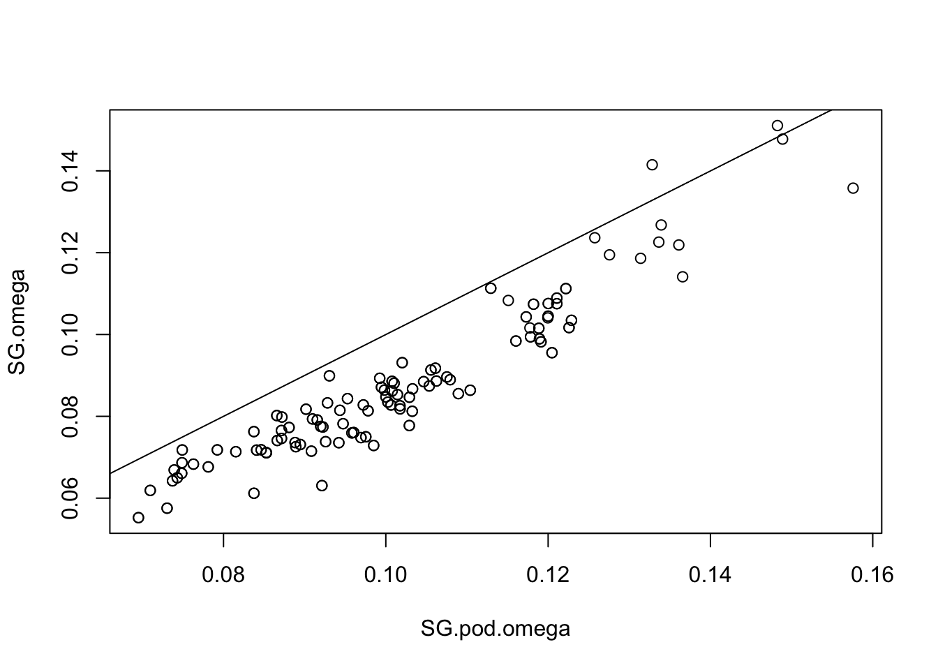
# Get the Forstner and Moonen Distance (FMD) between simulated and original posterior estimates (here a smaller value is better)
fmd.dist(SG.pod.omega,SG.omega)
## [1] 1.028579# Look at POD xtx values, and identify SNPs where the xtx values are above the 99% significance threshold from the POD. So in the plot, it is those loci (dots) which are above the abline
SG.pod.xtx=read.table("SG.BP.sim_summary_pi_xtx.out",h=T)$M_XtX
SG.pod.thresh=quantile(SG.pod.xtx,probs=0.99)
plot(SG.snp.res$M_XtX)
abline(h=SG.pod.thresh,lty=2)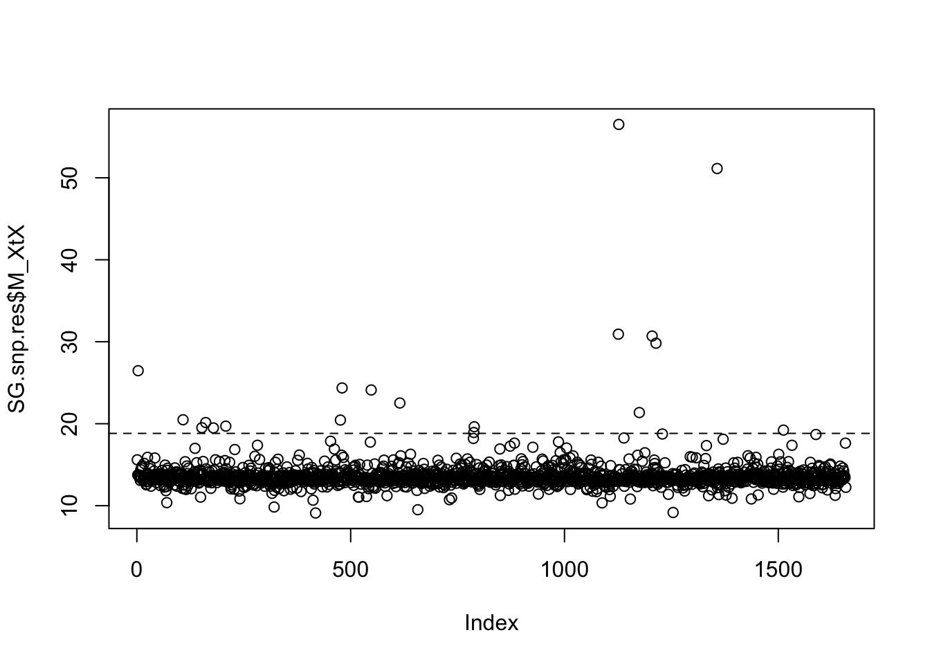
# Obtain the xtx threshold. Any SNPs with an xtx value greater than this are identified as outlier SNPs
SG.pod.thresh
## 99%
## 18.82108# Here I just saved the xtx values per SNP list, and then in excel/text editor filtered out the SNPs with an xtx greater than the threshold value as outliers.
SG.snp.scores <- as.data.frame(SG.snp.res$M_XtX)
write.table(SG.snp.scores, file="SG.snp.scores.txt", sep="\t")From here you can also run the auxiliary model in BayPass to identify outliers associated with environmental variables. To do this, you do not need to run the R code above, but rather simply run another version of the bash script, and identify outliers based on their Bayes Factor values (i.e. SNPs with dB > 20, from the dB column of the *_summary_betai_reg.out output file).
I hope this tutorial helps my fellow Pool-Seq peeps! I know there are probably more eloquent ways to run these analyses, but this should at least get the job done. As always, feel free to contact me if you have any questions :)
Happy analyzing!